

Photo by editor
# Introduction
Exploratory data analysis (EDA) is an important step before building deep data analysis processes or data-driven AI systems, such as those based on machine learning models. While fixing common, real-world data quality issues and inconsistencies is often deferred until later stages of the data pipeline, EDA is an excellent opportunity to detect these issues as early as possible.
Below, we compile a list of 7 Python tricks to apply to your initial EDA process, that is, by effectively identifying and fixing various data quality issues.
To illustrate these tricks, we will use an artificially generated employee dataset, into which we will deliberately inject a variety of data quality issues to illustrate how to detect and handle them. Before trying the tricks, make sure you copy and paste the following rendering code into your coding environment first:
import numpy as np
import pandas as pd
import matplotlib.pyplot as plt
import seaborn as sns

# PREAMBLE CODE THAT RANDOMLY CREATES A DATASET AND INTRODUCES QUALITY ISSUES IN IT
np.random.seed(42)

n = 1000

df = pd.DataFrame({
    "age": np.random.normal(40, 12, n).round(),
    "income": np.random.normal(60000, 15000, n),
    "experience_years": np.random.normal(10, 5, n),
    "department": np.random.choice(
        ("Sales", "Engineering", "HR", "sales", "Eng", "HR "), n
    ),
    "performance_score": np.random.normal(3, 0.7, n)
})

# Randomly injecting data issues to the dataset

# 1. Missing values
df.loc(np.random.choice(n, 80, replace=False), "income") = np.nan
df.loc(np.random.choice(n, 50, replace=False), "department") = np.nan

# 2. Outliers
df.loc(np.random.choice(n, 10), "income") *= 5
df.loc(np.random.choice(n, 10), "age") = -5

# 3. Invalid values
df.loc(np.random.choice(n, 15), "performance_score") = 7

# 4. Skewness
df("bonus") = np.random.exponential(2000, n)

# 5. Highly correlated features
df("income_copy") = df("income") * 1.02

# 6. Duplicated entries
df = pd.concat((df, df.iloc(:20)), ignore_index=True)

df.head()
# 1. Detection of missing values by heatmap
Whereas Python libraries have functions like Pandas It counts the number of missing values for each attribute in your dataset. isnull() The function thus plots white, barcode-like lines for each missing value throughout your dataset, arranged horizontally by attribute.
plt.figure(figsize=(10, 5))
sns.heatmap(df.isnull(), cbar=False)
plt.title("Missing Value Heatmap")
plt.show()

df.isnull().sum().sort_values(ascending=False)
Heatmap to detect missing values Photo by author
# 2. Removing duplicates
This trick is a classic: simple, yet very effective for counting the number of replicated instances (rows) in your dataset, which you can then apply to drop_duplicates() to remove them. By default, this function preserves the first occurrence of each duplicate row and discards the rest. However, this behavior can be modified, for example keep="last" Option to retain the last event instead of the first, or keep=False to get rid of all Fully replicated queues. The behavior to choose will depend on the needs of your particular problem.
duplicate_count = df.duplicated().sum()
print(f"Number of duplicate rows: {duplicate_count}")

# Remove duplicates
df = df.drop_duplicates()
# 3. Identifying outliers using the interquartile range method
The interquartile range (IQR) method is a statistical approach to support data that are far enough away from the rest of the points to be considered outliers or extreme values. This trick provides an implementation of the IQR method that can be replicated for various numerical attributes, such as “income”:
def detect_outliers_iqr(data, column):
    Q1 = data(column).quantile(0.25)
    Q3 = data(column).quantile(0.75)
    IQR = Q3 - Q1
    lower = Q1 - 1.5 * IQR
    upper = Q3 + 1.5 * IQR
    return data((data(column) < lower) | (data(column) > upper))

outliers_income = detect_outliers_iqr(df, "income")
print(f"Income outliers: {len(outliers_income)}")

# Optional: cap them
Q1 = df("income").quantile(0.25)
Q3 = df("income").quantile(0.75)
IQR = Q3 - Q1
lower = Q1 - 1.5 * IQR
upper = Q3 + 1.5 * IQR
df("income") = df("income").clip(lower, upper)
# 4. Managing conflicting categories
Unlike outliers, which are typically associated with numerical characteristics, inconsistent categories across variables can arise from a variety of factors, such as manual inconsistencies in names or domain-specific variations such as mass or lower case counts. Therefore, the correct approach to handling them may partly involve the subjects’ skill in deciding the right set of categories to be considered valid. This example applies category conflict management to department names that refer to the same department.
print("Before cleaning:")
print(df("department").value_counts(dropna=False))

df("department") = (
    df("department")
    .str.strip()
    .str.lower()
    .replace({
        "eng": "engineering",
        "sales": "sales",
        "hr": "hr"
    })
)

print("\nAfter cleaning:")
print(df("department").value_counts(dropna=False))
# 5. Checking and validating limits
While outliers are statistically outlying values, outliers depend on domain-specific constraints, such as the values of the “age” attribute cannot be negative. This example identifies negative values for the “age” attribute and replaces them with null – notice that these invalid values are converted to missing values, so a downstream strategy will also be required to deal with them.
invalid_age = df(df("age") < 0)
print(f"Invalid ages: {len(invalid_age)}")

# Fix by setting to NaN
df.loc(df("age") < 0, "age") = np.nan
# 6. Application of log transform to skewed data
In our example dataset, skewed data attributes such as “bonuses” are usually better transformed into something that resembles a normal distribution, as this facilitates the majority of downstream machine learning analyses. This trick applies a log transformation, showing the before and after characteristics of our data.
skewness = df("bonus").skew()
print(f"Bonus skewness: {skewness:.2f}")

plt.hist(df("bonus"), bins=40)
plt.title("Bonus Distribution (Original)")
plt.show()

# Log transform
df("bonus_log") = np.log1p(df("bonus"))

plt.hist(df("bonus_log"), bins=40)
plt.title("Bonus Distribution (Log Transformed)")
plt.show()
Before log transformation | Photo by author
After log transformation | Photo by author
# 7. Detection of redundant features by correlation matrix
We wrap up this list the same way we started: with visual communication. Correlation matrices expressed as heatmaps help identify pairs of features that are highly correlated—a strong indication that they may contain redundant information that is often minimized in subsequent analysis. In this example, the most highly associated pairs of attributes are also printed for further interpretation:
corr_matrix = df.corr(numeric_only=True)

plt.figure(figsize=(10, 6))
sns.heatmap(corr_matrix, annot=True, fmt=".2f", cmap="coolwarm")
plt.title("Correlation Matrix")
plt.show()

# Find high correlations
high_corr = (
    corr_matrix
    .abs()
    .unstack()
    .sort_values(ascending=False)
)

high_corr = high_corr(high_corr < 1)
print(high_corr.head(5))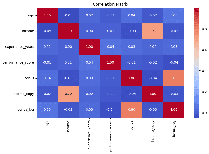
Correlation matrix to detect redundant features Photo by author
# wrap up
With the list above, you’ve learned 7 useful tricks to get the most out of your exploratory data analysis, helping you uncover and deal with a variety of data quality issues and discrepancies effectively and intuitively.
Ivan Palomares Carrascosa Is a leader, author, speaker, and consultant in AI, Machine Learning, Deep Learning, and LLMS. He trains and guides others in real-world applications of AI.