Finding heavy traffic indicators on I-94

https://www.youtube.com/watch?v=4uhye1sqp8

In this project walkthrough, we will discover how to use data vessel techniques to expose traffic samples at Interstate 94, one of the busiest highways in the United States. By analyzing the weather conditions and time -based factors as well as real -world traffic volume data, we will identify the key indicators of heavy traffic that can help passengers plan their travel hours more efficiently.

Traffic crowds are a daily challenge for millions of passengers. Understanding why and why heavy traffic is there can help drivers make informed decisions about their travel hours, and can help the city’s planners improve traffic flow. Through this hands -on analysis, we will discover amazing samples that are beyond clear expectations of the rush times.

During this tutorial, we will create more than one image .They that tells a comprehensive story about traffic samples, which shows how the concept of research data can show insights that only abstract data can be lost.

Will you learn

By the end of this tutorial, you will know how:

• Make and translate them to understand the distribution of traffic volume
• Use Time series concepts to identify daily, weekly and monthly patterns
• Create side -by -side plot for efficient comparison
• Analyze the connection between weather conditions and the volume of traffic
• Apply grouping and collecting techniques for time -based analysis
• Multiple concepts to tell a full data story. Combine types of types

Before you start: Pre -instruction

To take the maximum of this project, follow these initial steps:

1. Review the project

   Get access to the project and familiarize yourself with goals and structures: searching for heavy traffic indicator projects.

2. Access the solution notebook

   You can see it here and download to see what we will cover: Solution notebook

3. Prepare your environment

   • If you are using the Data Quest platform, everything has already been configured for you
   • If working locally, make sure you have a pandas, metaplatlib, and marine borne
   • Download from dataset UCI Machine Learning Repeatory

4. Provisions

New in Mark Dowan? We recommend learning the basics to format the header and adding context to your Japter notebook: Mark Dowan Guide.

To set your environment

Let’s start by importing the necessary libraries and loading your dataset:

import pandas as pd
import matplotlib.pyplot as plt
import seaborn as sns
%matplotlib inline

%matplotlib inline Command is a magic that offers our plots directly in the notebook. This interactive data is essential for exploration work flu.

traffic = pd.read_csv('Metro_Interstate_Traffic_Volume.csv')
traffic.head()

   holiday   temp  rain_1h  snow_1h  clouds_all weather_main  \
0      NaN  288.28      0.0      0.0          40       Clouds
1      NaN  289.36      0.0      0.0          75       Clouds
2      NaN  289.58      0.0      0.0          90       Clouds
3      NaN  290.13      0.0      0.0          90       Clouds
4      NaN  291.14      0.0      0.0          75       Clouds

      weather_description            date_time  traffic_volume
0      scattered clouds  2012-10-02 09:00:00            5545
1        broken clouds  2012-10-02 10:00:00            4516
2      overcast clouds  2012-10-02 11:00:00            4767
3      overcast clouds  2012-10-02 12:00:00            5026
4        broken clouds  2012-10-02 13:00:00            4918

With the weather conditions for every hour in our dataset, the Westbound I-94 measures the traffic volume per hour from the station between Manipolis and St. Paul. Key columns include:

• Holiday: Holiday name (if applicable)
• Temporary: Temperature in Calvin
• Rain_1: Rain in mm for an hour
• Snow_1 h: Snow in mm for an hour
• Cloud_al: Percentage of cloud cover
• The weather_man: The normal weather category
• Weather_: Detailed detail of the weather
• History_ Time: Time stamp of measurement
• Traffic_Olom: Number of vehicles (our target variable)

Learning insights: Notice that the temperature is in the calf (about 288k = 15 ° C = 59 ° F). It is unusual for everyday use but is common in scientific datases. When the results in front of the stakeholders, you want to transform them into a foreign height or a cells.

Search for initial data

Before diving into concepts, let’s understand our dataset structure:

traffic.info()

RangeIndex: 48204 entries, 0 to 48203
Data columns (total 9 columns):
 #   Column               Non-Null Count  Dtype
---  ------               --------------  -----
 0   holiday              61 non-null     object
 1   temp                 48204 non-null  float64
 2   rain_1h              48204 non-null  float64
 3   snow_1h              48204 non-null  float64
 4   clouds_all           48204 non-null  int64
 5   weather_main         48204 non-null  object
 6   weather_description  48204 non-null  object
 7   date_time            48204 non-null  object
 8   traffic_volume       48204 non-null  int64
dtypes: float64(3), int64(2), object(4)
memory usage: 3.3+ MB

We have about 50 50,000 hours observations spanning many years. Note that only 61 out of 48,204 rows in the holiday column are non -noble values. Let’s investigate:

traffic('holiday').value_counts()

holiday
Labor Day                    7
Christmas Day                6
Thanksgiving Day             6
Martin Luther King Jr Day    6
New Years Day                6
Veterans Day                 5
Columbus Day                 5
Memorial Day                 5
Washingtons Birthday         5
State Fair                   5
Independence Day             5
Name: count, dtype: int64

Learning insights: At first glance, you think the holiday column is closely useless with very few values. But in fact, the holidays are only marked at midnight during the holidays. This is an excellent example of how to understand your data structure can make a big difference: the data that looks like a lost data can in fact be a deliberate design. For a complete analysis, you want to extend these holiday markers to cover 24 hours of every holiday.

Let’s check our numeric variants:

traffic.describe()

              temp       rain_1h       snow_1h    clouds_all  traffic_volume
count  48204.000000  48204.000000  48204.000000  48204.000000    48204.000000
mean     281.205870      0.334264      0.000222     49.362231     3259.818355
std       13.338232     44.789133      0.008168     39.015750     1986.860670
min        0.000000      0.000000      0.000000      0.000000        0.000000
25%      272.160000      0.000000      0.000000      1.000000     1193.000000
50%      282.450000      0.000000      0.000000     64.000000     3380.000000
75%      291.806000      0.000000      0.000000     90.000000     4933.000000
max      310.070000   9831.300000      0.510000    100.000000     7280.000000

Key observations:

• The temperature is from 0k to 310k (that 0k is suspicious and is likely to have data quality problem)
• There is no rain in most hours (75th percent for both rain and snow is 0)
• Traffic volume occurs from 0 to 7,280 vehicles per hour
• Mid -3,260 and median (3,380) traffic volumes are the same, which suggest relatively harmony.

Concept of distribution of traffic volume

Let’s make your first concept to understand the traffic patterns:

plt.hist(traffic("traffic_volume"))
plt.xlabel("Traffic Volume")
plt.title("Traffic Volume Distribution")
plt.show()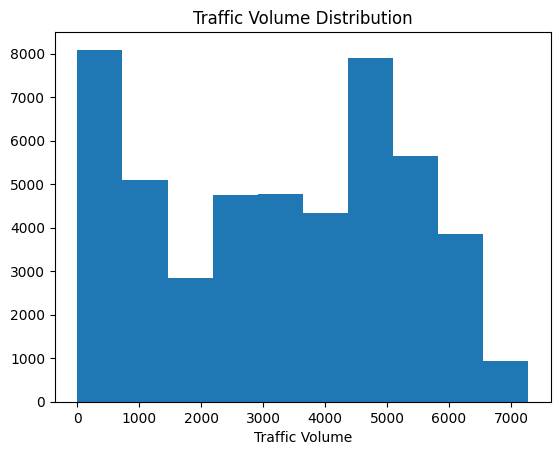

Learning insights: Always label your axis and add titles! Your audience should not know what they are seeing. Without context, the graph is just beautiful color.

Hastagram has revealed an amazing bummodel distribution with two separate peaks.

• A peak near 0-1,000 vehicles (lower traffic)
• Another peak approximately 4,000-5,000 vehicles (high traffic)

This proposes two separate traffic governments. My immediate assumption: These are according to day and night traffic samples.

Day vs Night Analysis

Let’s test your assumptions by dividing the data into day and night periods:

# Convert date_time to datetime format
traffic('date_time') = pd.to_datetime(traffic('date_time'))

# Create day and night dataframes
day = traffic.copy()((traffic('date_time').dt.hour >= 7) &
                     (traffic('date_time').dt.hour < 19))

night = traffic.copy()((traffic('date_time').dt.hour >= 19) |
                       (traffic('date_time').dt.hour < 7))

Learning Insight: I chose “Day” times from 7pm to 7pm, which gives us a period of 12 hours. This is somewhat arbitrary and you can explain different rush times. I encourage you to experience with different definitions, such as 6am to 6pm, and see how it affects your results. Avoid eliminating your analysis, just keep periods balanced.

Now imagine both of us as well as:

plt.figure(figsize=(11,3.5))

plt.subplot(1, 2, 1)
plt.hist(day('traffic_volume'))
plt.xlim(-100, 7500)
plt.ylim(0, 8000)
plt.title('Traffic Volume: Day')
plt.ylabel('Frequency')
plt.xlabel('Traffic Volume')

plt.subplot(1, 2, 2)
plt.hist(night('traffic_volume'))
plt.xlim(-100, 7500)
plt.ylim(0, 8000)
plt.title('Traffic Volume: Night')
plt.ylabel('Frequency')
plt.xlabel('Traffic Volume')

plt.show()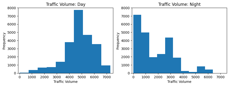

Full! Our assumptions have been confirmed. Low traffic peaks are fully compatible with night hours, while high traffic peaks are during the day. Consider how I set the limits of the same axis for both plots – this ensures proper visual comparisons.

Let’s correct the amount of this difference:

print(f"Day traffic mean: {day('traffic_volume').mean():.0f} vehicles/hour")
print(f"Night traffic mean: {night('traffic_volume').mean():.0f} vehicles/hour")

Day traffic mean: 4762 vehicles/hour
Night traffic mean: 1785 vehicles/hour

The day traffic is 3x more than the average night traffic!

Monthly traffic samples

Let’s look for seasonal patterns by checking traffic for months:

day('month') = day('date_time').dt.month
by_month = day.groupby('month').mean(numeric_only=True)

plt.plot(by_month('traffic_volume'), marker='o')
plt.title('Traffic volume by month')
plt.xlabel('Month')
plt.show()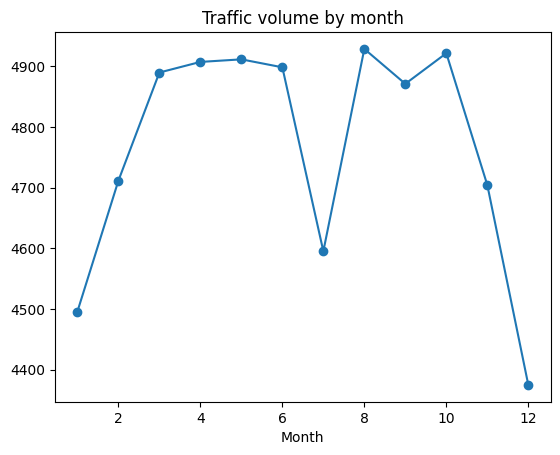

Plot shows:

• Winter Months (January, February, November, Dec) specially traffic is low
• A dramatic dip in July that seems unusual

Let’s investigate that the irregularities in July:

day('year') = day('date_time').dt.year
only_july = day(day('month') == 7)

plt.plot(only_july.groupby('year').mean(numeric_only=True)('traffic_volume'))
plt.title('July Traffic by Year')
plt.show()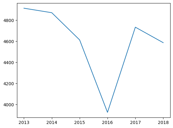

Learning insights: This is a great example of why the Exploroory concept is so valuable. Dip that July? This shows that I-94 was completely closed for several days in July 2016. These zero traffic days draw a monthly average dramatic way. This is a reminder that outlaits can significantly affect this so always investigate unusual patterns in your data!

The day of the week’s samples

Let’s check weekly samples:

day('dayofweek') = day('date_time').dt.dayofweek
by_dayofweek = day.groupby('dayofweek').mean(numeric_only=True)

plt.plot(by_dayofweek('traffic_volume'))

# Add day labels for readability
days = ('Mon', 'Tue', 'Wed', 'Thu', 'Fri', 'Sat', 'Sun')
plt.xticks(range(len(days)), days)
plt.xlabel('Day of Week')
plt.ylabel('Traffic Volume')
plt.title('Traffic by Day of Week')
plt.show()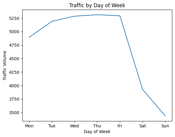

Clear Sample: The weekly traffic is significantly higher than the weekend traffic. It aligns with traveling samples as most people try to work from Monday to Friday.

Samples per hour: Saturday’s weekend vs weekend

Let’s compare the weekly business days, dig deep into the hourly patterns:

day('hour') = day('date_time').dt.hour
business_days = day.copy()(day('dayofweek') <= 4)  # Monday-Friday
weekend = day.copy()(day('dayofweek') >= 5)        # Saturday-Sunday

by_hour_business = business_days.groupby('hour').mean(numeric_only=True)
by_hour_weekend = weekend.groupby('hour').mean(numeric_only=True)

plt.figure(figsize=(11,3.5))

plt.subplot(1, 2, 1)
plt.plot(by_hour_business('traffic_volume'))
plt.xlim(6,20)
plt.ylim(1500,6500)
plt.title('Traffic Volume By Hour: Monday–Friday')

plt.subplot(1, 2, 2)
plt.plot(by_hour_weekend('traffic_volume'))
plt.xlim(6,20)
plt.ylim(1500,6500)
plt.title('Traffic Volume By Hour: Weekend')

plt.show()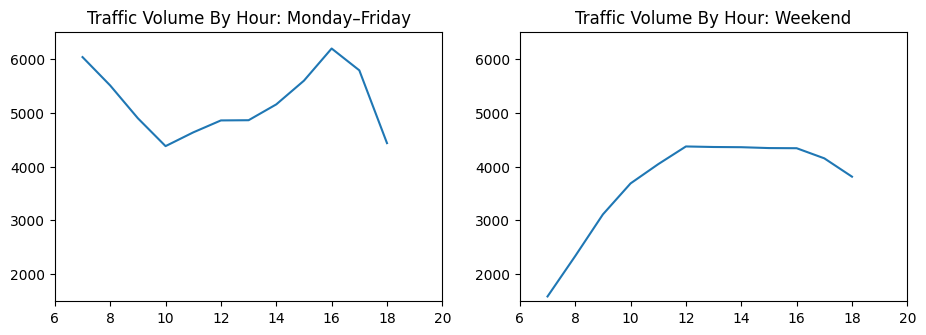

The samples are surprisingly different:

• The day of the week: Clean morning (7 am) and evening (4-5 pm) peaks of rush time
• The weekend: A gradual increase in the day without any separate peaks
• The best time to travel the day of the week: 10 o’clock in the morning (between rush times)

Analyzing the effects of the weather

Now let’s see if the weather conditions affect the traffic:

weather_cols = ('clouds_all', 'snow_1h', 'rain_1h', 'temp', 'traffic_volume')
correlations = day(weather_cols).corr()('traffic_volume').sort_values()
print(correlations)

clouds_all       -0.032932
snow_1h           0.001265
rain_1h           0.003697
temp              0.128317
traffic_volume    1.000000
Name: traffic_volume, dtype: float64

Surprisingly weakening of connection! It seems that the weather does not significantly affect the traffic volume. The temperature shows the strongest connection at only 13 %.

Let’s imagine it with a plot scattered:

plt.figure(figsize=(10,6))
sns.scatterplot(x='traffic_volume', y='temp', hue='dayofweek', data=day)
plt.ylim(230, 320)
plt.show()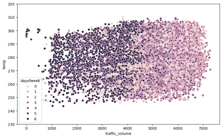

Learning insights: When I first prepared this secretary plot, I was very excited to see separate clusters. Then I noticed that the colors are only consistent with our previous search. This is a reminder that always think about criticism what the samples mean, not just what they are present!

Let’s review the specific conditions of the weather:

by_weather_main = day.groupby('weather_main').mean(numeric_only=True).sort_values('traffic_volume')

plt.barh(by_weather_main.index, by_weather_main('traffic_volume'))
plt.axvline(x=5000, linestyle="--", color="k")
plt.show()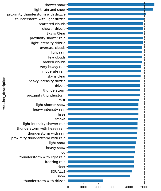

The vision of learning: This is an important lesson of data analysis and you should always test the size of your sample! These weather conditions with seemingly high traffic volume? They have only 1-4 data points. You cannot draw reliable conclusions from such small samples. The most common weather conditions (clean sky, scattered clouds) contain thousands of data points and show the average traffic level.

Key results and results

Through our research vision, we have discovered:

Heavy traffic time -based indicators:

1. The day vs. night: Day time (7am to 7 am in the morning) 3x more traffic than night time
2. The day of the week: The day of the week is significantly higher traffic than the weekend
3. Rush times: Saturday 7-8 pm and evening 4-5p show the most volumes
4. Seasonal: In the winter months (January, February, November, December) the amount of traffic decreases

The weather effect:

• Amazingly minimal concrete between weather and traffic volume
• The temperature shows the weak positive implication (13 %)
• No conduct of rain and snow shows
• This shows that passengers are driving without weather conditions

Best time to travel:

• To avoid: Saturday’s rush times (7-8 pm, 4-5 pm)
• Maximum: Weekends, nights, or day of the week (near 10 am) mid -day

Next steps

To enhance this analysis, consider:

1. Holiday analysis: Expand holiday markers to cover all 24 hours and analyze holiday traffic samples
2. The perseverance of the weather: Does continuous hours of rain/snow affect the traffic differently?
3. Outline investigations: Deep in the shutdown of July 2016 and other irregularities
4. Modeling predicted: Create a model to predict the volume of traffic on time and weather
5. Directional analysis: Compare the Eastbound vs Westbound traffic samples

This project shows the strength of research ventilation. We started with a simple question, “What happens because of heavy traffic?” And through a systematic manner, exposed clear patterns. Weather searches surprised me. I expected to significantly affect traffic from rain and snow. It reminds us to let the data challenge our assumptions!

Beautiful graphs are good, but they are not a matter of it. The actual value of the search data analysis comes when you really dig into the Enough to understand what is happening in your data based on what you get, based on what you get. Whether your passenger is planning your way or improving traffic flow, this insight provides viable intelligence.

If you let this project go, please share your results in this Data Quest Community And tag me (Anna_strahl). I would love to see which samples you discover!

Happy Analysis!