
Photo by author
# Introduction
When applying for a job at Meta (formerly Facebook), Apple, Amazon, Netflix, or Alphabet (Google)—collectively known as the FAANG—interviewers rarely test whether you can read textbook definitions. Instead, interviewers want to see if you critically analyze data and if you’ll spot bad analysis before sending it into production. Statistical traps are one of the most reliable ways to test this.
![]()
These pitfalls mimic the decisions analysts face on a daily basis: a dashboard number that looks good but is actually misleading, or an experiment result that looks plausible but has a structural flaw. The interviewer already knows the answer. What they’re looking at is your thought process, including whether you ask the right questions, notice missing information, and fall back on a number that looks good at first glance. Candidates stumble over these pitfalls again and again, even those with a strong mathematical background.
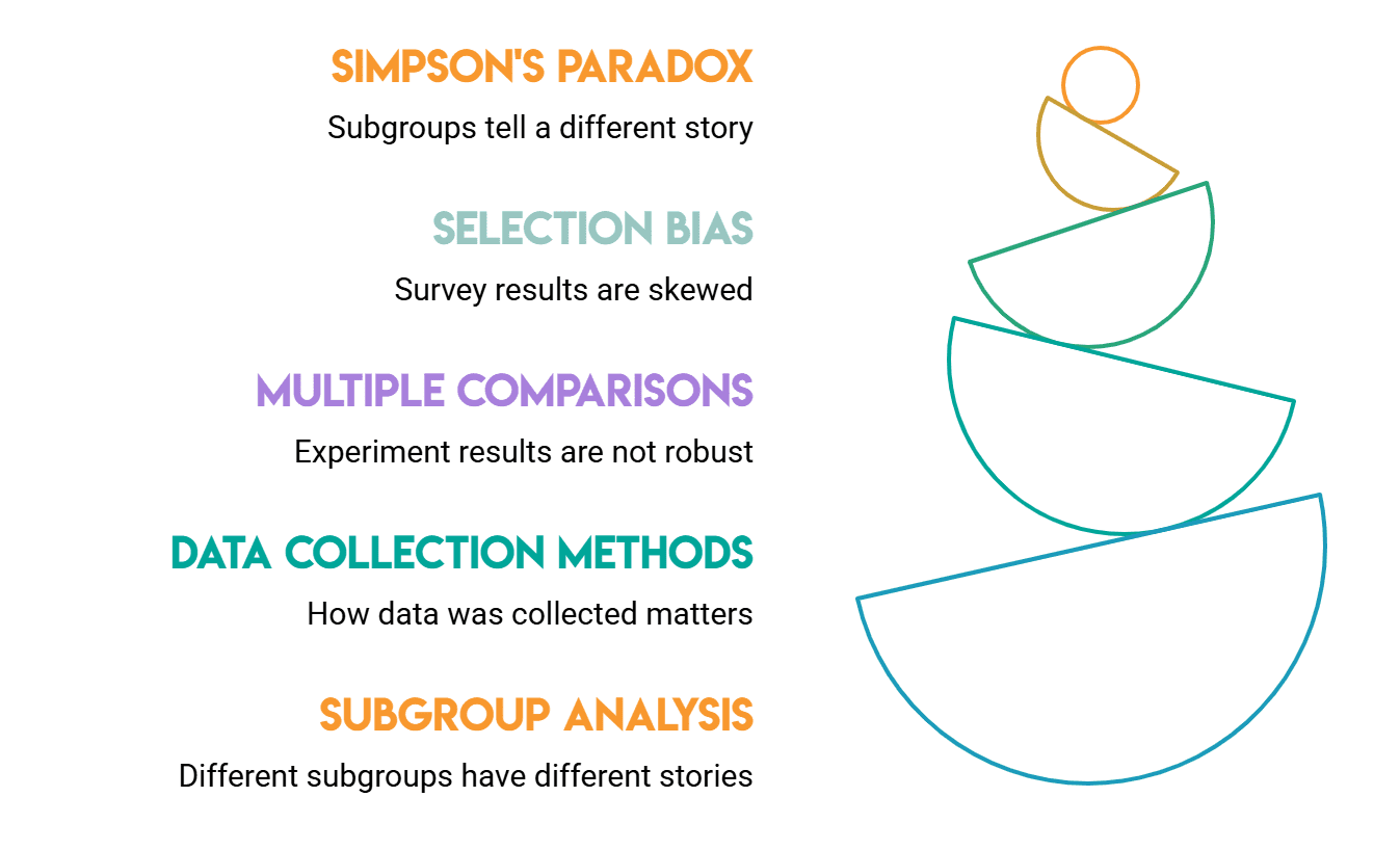
We will examine five of the most common pitfalls.
# Understanding Simpson’s Paradox
The purpose of this trap is to catch people who unquestioningly trust aggregate numbers.
Simpson’s paradox occurs when a trend appears in different groups of data but disappears or reverses when the groups are combined. The best example of this is UC Berkeley’s 1973 admissions data: overall admission rates favored men, but when broken down by department, women’s admission rates were equal or better. The overall numbers were misleading because women applied to more competitive departments.
Contrast is inevitable whenever groups are of different sizes and have different base rates. This understanding is what can separate a superficial response from a deeper response.
In interviews, a question might look like this: “We ran an A/B test. Overall, variant B had a higher conversion rate. However, when we break it down by device type, variant A performed better on both mobile and desktop. What’s going on?” A strong candidate cites Simpson’s paradox, explains its cause (group proportions differ between two variances), and asks to look at the variance rather than relying on aggregate data.
Interviewers use this to test whether you naturally ask about subgroup distributions. If you only report the total number, your points are gone.
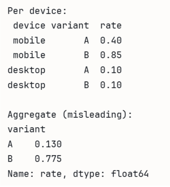
// Demonstrating with A/B test data
In the following demonstration using Panda.we can see how the aggregate rate can be misleading.
import pandas as pd

# A wins on both devices individually, but B wins in aggregate
# because B gets most traffic from higher-converting mobile.
data = pd.DataFrame({
    'device':   ('mobile', 'mobile', 'desktop', 'desktop'),
    'variant':  ('A', 'B', 'A', 'B'),
    'converts': (40, 765, 90, 10),
    'visitors': (100, 900, 900, 100),
})
data('rate') = data('converts') / data('visitors')

print('Per device:')
print(data(('device', 'variant', 'rate')).to_string(index=False))
print('\nAggregate (misleading):')
agg = data.groupby('variant')(('converts', 'visitors')).sum()
agg('rate') = agg('converts') / agg('visitors')
print(agg('rate'))
Output:
# Identifying selection bias
This test lets interviewers gauge whether you think about where data comes from before analyzing it.
Selection bias occurs when the data you have is not representative of the population you are trying to understand. Because the bias is in the data collection process rather than the analysis, it is easy to overlook.
Consider these possible interview framings:
- We analyzed our customer survey and found that 80% are satisfied with the product. Does it tell us that our product is good? A solid candidate will indicate that satisfied customers are more likely to respond to a survey. The 80% figure likely overstates satisfaction because unhappy customers choose not to participate.
- We examined customers who left last quarter and discovered that they had essentially poor engagement scores. Should we focus on engagement to reduce engagement? The problem here is that you only have engagement data for engaged users. You don’t have engagement data for users who stay, making it impossible to know whether low engagement actually predicts churn or is just a characteristic of churn users in general.
A related type worth knowing is survivorship bias: you only observe results that made it through some filter. If you only use data from successful products to analyze why they succeeded, you’re ignoring those that failed for the same reasons you see as strengths.
// Simulated survey non-response
We can simulate how using non-response bias biases the results. NumPy.
import numpy as np
import pandas as pd

np.random.seed(42)
# Simulate users where satisfied users are more likely to respond
satisfaction = np.random.choice((0, 1), size=1000, p=(0.5, 0.5))
# Response probability: 80% for satisfied, 20% for unsatisfied
response_prob = np.where(satisfaction == 1, 0.8, 0.2)
responded = np.random.rand(1000) < response_prob

print(f"True satisfaction rate: {satisfaction.mean():.2%}")
print(f"Survey satisfaction rate: {satisfaction(responded).mean():.2%}")
Output:
![]()
Interviewers use selection bias questions to see if you separate “what the data shows” from “what is true about consumers.”
# Prevention of hacking
P-hacking (also known as data dredging) occurs when you run many tests and only report tests with \( p < 0.05 \). The problem is that the \( p \) values are only for individual tests. If 20 tests are run at the 5% significance level, one false positive would be expected by chance. The false discovery rate is increased by fishing for a significant result. An interviewer might ask you the following: "Last quarter, we ran fifteen feature tests. At \( p < 0.05 \), three were found to be significant. Do all three need to be shipped?" A weak answer says yes. A strong answer would first ask what the hypotheses were before running the test, if significance thresholds were predetermined, and whether the team corrected for multiple comparisons. Follow-up often includes how you will design experiments to avoid this. Preregistering hypotheses before data collection is the most direct solution, because it removes the option of deciding after the fact which tests were "real."
// Seeing false positives accumulate
We can observe how false positives are used by chance. SciPy.
import numpy as np
from scipy import stats
np.random.seed(0)

# 20 A/B tests where the null hypothesis is TRUE (no real effect)
n_tests, alpha = 20, 0.05
false_positives = 0

for _ in range(n_tests):
    a = np.random.normal(0, 1, 1000)
    b = np.random.normal(0, 1, 1000)  # identical distribution!
    if stats.ttest_ind(a, b).pvalue < alpha:
        false_positives += 1

print(f'Tests run:                 {n_tests}')
print(f'False positives (p<0.05): {false_positives}')
print(f'Expected by chance alone: {n_tests * alpha:.0f}')
Output:
![]()
Even with zero true effect, ~1 \(p < 0.05 \) in 20 tests clears chance. If a team performs 15 experiments and reports only the significant ones, those results are mostly noise. It is equally important to understand exploratory analysis as a form of hypothesis generation rather than confirmation. Before anyone takes action based on search results, a confirmatory experiment is required.
# Multiple testing arrangements
This test is closely related to p-hacking, but is worth understanding on its own.
The multiple testing problem is a formal statistical problem: when you run several hypothesis tests at once, the probability of at least one false positive increases exponentially. Even if the treatment has no effect, if you test 100 metrics in an A/B test and declare any with \( p < 0.05 \) as significant, you should estimate about five false positives. His corrections are well known: Bonferroni correction (divide alpha by the number of tests) and Benjamini-Hochberg (controls the false discovery rate rather than the family-wise error rate).
Bonferroni is a conservative approach: for example, if you test 50 metrics, your threshold per test drops to 0.001, making it difficult to detect true effects. Benjamini-Hochberg is more appropriate when you are willing to accept some false positives in exchange for more statistical power.
In interviews, this comes up when discussing how the company tracks experience metrics. A question might be: “We monitor 50 metrics per experiment. How do you decide which ones matter?” A concrete answer argues for pre-defining primary metrics before the experiment runs and treating secondary metrics as exploratory, acknowledging the problem of multiple testing.
Interviewers are trying to find out if you know that taking more tests is more noise than more information.
# Resolving conflicting variables
This trap catches candidates who consider correlation to be causal without asking what else might explain the correlation.
Oh Confounding variables One that affects both the independent and dependent variables, creating the illusion of a direct relationship where none exists.
Best example: Ice cream sales and sink rates are correlated, but the confounder is summer heat. Both go up in the warmer months. Acting on this correlation without accounting for confounders leads to poor judgments.
Confounding is particularly dangerous in observational data. Unlike a randomized experiment, observational data do not distribute potential confounders equally between groups, so the difference you see may not be due to the variable you are studying.
A typical interview sequence is: “We noticed that users who use our mobile app more often have significantly higher revenue. Should we push notifications to increase app opens?” A weak candidate says yes. A strong person asks what type of user opens the app most often to begin with: possibly the most engaged, highest-value users.
Engagement drives both app opens and spending. App opening is not generating revenue. They symbolize the same basic consumer quality.
Interviewers use confounding to test whether you separate causality before drawing conclusions, and whether you will emphasize the similarity of random experiments or propensity scores before recommending action.
// Simulating a tangled relationship
import numpy as np
import pandas as pd
np.random.seed(42)
n = 1000
# Confounder: user quality (0 = low, 1 = high)
user_quality = np.random.binomial(1, 0.5, n)
# App opens driven by user quality, not independent
app_opens = user_quality * 5 + np.random.normal(0, 1, n)
# Revenue also driven by user quality, not app opens
revenue = user_quality * 100 + np.random.normal(0, 10, n)
df = pd.DataFrame({
    'user_quality': user_quality,
    'app_opens': app_opens,
    'revenue': revenue
})
# Naive correlation looks strong — misleading
naive_corr = df('app_opens').corr(df('revenue'))
# Within-group correlation (controlling for confounder) is near zero
corr_low  = df(df('user_quality')==0)('app_opens').corr(df(df('user_quality')==0)('revenue'))
corr_high = df(df('user_quality')==1)('app_opens').corr(df(df('user_quality')==1)('revenue'))
print(f"Naive correlation (app opens vs revenue): {naive_corr:.2f}")
print(f"Correlation controlling for user quality:")
print(f"  Low-quality users:  {corr_low:.2f}")
print(f"  High-quality users: {corr_high:.2f}")
Output:
Naive correlation (app opens vs revenue): 0.91

Correlation controlling for user quality:

Low-quality users:  0.03
High-quality users: -0.07
Bid number looks like a strong signal. Once you overcome the confounder, it disappears completely. Interviewers who see a candidate running such a stratified check (rather than accepting the aggregate relationship) know they’re talking to someone who won’t send a broken recommendation.
# wrap up
All five of these traps have something in common: they require you to slow down and question what the numbers show at first glance before accepting the data. Interviewers use these scenarios specifically because your first instinct is often wrong, and the depth of your response after that first instinct is what separates a candidate from someone who can work independently and needs direction on every analysis.
None of these ideas are difficult to understand, and interviewers tend to inquire about them because they are common failure modes in real data work. A candidate who recognizes Simpson’s paradox in product metrics, captures selection bias in surveys, or questions whether an experiment result survives multiple comparisons is the one who will send fewer bad judgments.
If you go in. Fang Interview with the reflex to ask the following questions, you are already ahead of most candidates:
- How was this data collected?
- Are there subgroups that tell a different story?
- How many tests contributed to this result?
In addition to helping in interviews, these habits can also prevent bad decisions from reaching production.
Net Rosiedi A data scientist and product strategist. He is also an adjunct professor teaching analytics, and the founder of StrataScratch, a platform that helps data scientists prepare for their interviews with real interview questions from top companies. Nate writes on the latest trends in the career market, gives interview advice, shares data science projects, and covers all things SQL.