


Photo by author
# Setup
You are about to train a model when you find that 20% of your values are missing. Do you skip these rows? Fill them with average? Use something fancier? The answer matters more than you think.
If you Google it, you’ll find dozens of optimization methods, from the dead simple (use the mean) to the sophisticated (iterative machine learning models). You think fancy methods are better. knn Considers similar rows. Mice Builds predictive models. They should just do better by slapping the average, right?
We thought so too. We were wrong.
# Experience
We caught up Crop recommendation dataset From StrataScience Projects – 2200 soil samples from 220 crops, with characteristics such as nitrogen levels, temperature, moisture and rainfall. A random forest hits this object with 99.6% accuracy. It’s almost suspiciously clean.
This analysis extends our Analysis of agricultural data project, which explores the same dataset through EDA and statistical testing. Here, we ask: What happens when clean data meets a real-world problem – missing values?
Best for our experience.
We introduced 20% missing values (completely random, simulating sensor failures), then tested five failure modes:

Our testing was complete. We used 10-fold cross-validation in five random seeds (total of 50 runs in each procedure). To ensure that no information leaked from the test set into the training set, our imputation models were trained only on the training sets. For our statistical tests, we applied the Bonferroni correction. We also normalized the input features for both KN and mice, as if we had not normalized them, when calculating distances for these methods an input with values between 0 and 300 (rainfall) would have a greater effect than a range of 3 to 10 (pH). We have full code and reproduction results available Notebook.
Then we ran it and stared at the results.
# surprise
Here’s what we expected: KNNs or rats would win, because they’re smart. They consider the relationships between features. They use actual machine learning.
Here’s what we got:

The median and mean are tied for first place. Sophisticated methods came third and fourth.
We ran a statistical test. Mean versus median: P = 0.7. Not even close to important. They are effectively the same.
But here’s the kicker: they both significantly outperformed KNs and mice (P < 0.001 after Bonferroni correction). The simple methods just didn't match the fancy ones. They beat them.
# wait, what?
Before you throw out your mice installation, let’s dig into why this happened.
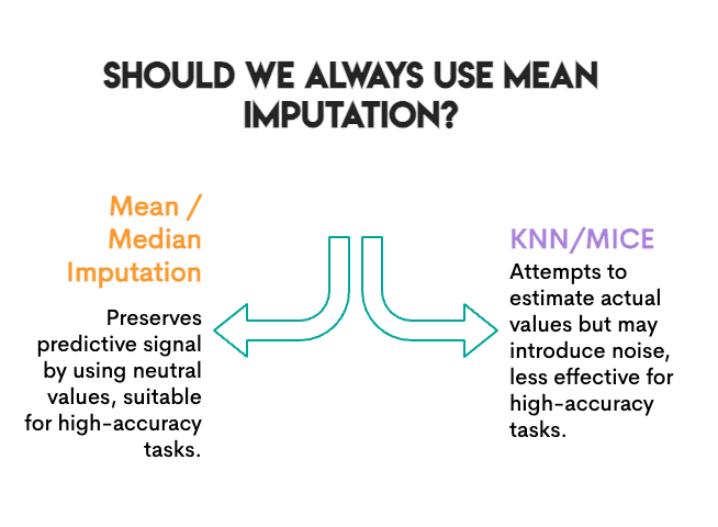
The work was predictable. We measured accuracy. Does the model still classify crops correctly after classification? For this particular purpose, what is important is to preserve the predictive signal, not necessarily the exact values.
This means something interesting: it replaces missing values with a “neutral” value that does not bias the model towards a particular class. It’s boring, but it’s safe. A random forest can still find its decision limits.
Try KNN and mice as much as possible. They estimate what the actual value might be. But in doing so, they can introduce noise. If the nearest neighbors don’t match, or if the iterative modeling of the mice picked faster samples, you’ll be adding error rather than removing it.
The baseline was already high. At 99.6% accuracy, this is a very simple classification problem. When the signal is strong, the stigma errors are less important. The model can tolerate some noise.
Random forest is strong Tree-based models handle incomplete data well. A linear model struggled more with distorting mean regression variance.
Not so fast.
# Plot twist
We measured something else: correlation conservation.
Here’s the thing about real data: Features don’t exist in isolation. They go together. In our dataset, when soil has more phosphorus, it generally has more potassium (correlation of 0.74). This is not random. Growers usually add these nutrients together, and some soil types maintain both.
When you eliminate missing values, you can accidentally break these relationships. Regardless of whether it looks like phosphorus in this array. Do this long enough, and the relationship between P and K starts to break down. Your generated data may look fine column by column, but the relationships between the columns are quietly falling apart.
Why does it matter? If your next step is Clusteringfor , for , for , . PCAor any analysis where attribute relationships are the point, you’re working with corrupted data and don’t know it.
We examined: How much of this peak correlation survived after the exception?

Photo by author
The hierarchy was completely reversed.
KNN preserved correlation perfectly. The mean and median destroyed a quarter of that. And random sampling (which samples values independently for each column) eliminated the relationship.
It makes sense. Mean imputation replaces missing values with the same number regardless of what the other features look like. If a row has more nitrogen, it doesn’t care. It still enforces average potassium. KNN looks at similar rows, so if high N rows are of high K, it will end up with a high K value.
# off trade
Here’s the real find: There is no one-best contrast method. Instead, choose the most appropriate method based on your specific purpose and context.
Accuracy rating and correlation rating are almost opposite:

Photo by author
(At least the random sample is consistent – it’s bad at everything.)
This trade-off is not unique to our dataset. It’s baked into how these methods work. The mean/median are univariate, and they look at one column at a time. KNNs/rats are multivariate, and they understand relationships. Univariate methods preserve normal distributions but eliminate correlation. Multivariate methods preserve structure and may introduce some forms of prediction error/noise.
# So, what exactly should you do?
After running this experiment and digging through the literature, here’s our practical guide:
Use the mean or median when:
- Your goal is prediction (classification, regression).
- You are using a robust model (random forest, xg boost, neural net).
- The missing rate is less than 30%
- You need something fast
Use KNN when:
- You need to preserve attribute relationships
- The downstream task is clustering, PCA, or visualization
- You want correlations to survive for investigative analysis
Use mice when:
- You need accurate standard errors (for statistical estimates).
- You are reporting confidence intervals or p values
- The missing data mechanism can be mar (missing at random).
Avoid random samples:
- It is attractive because it “preserves distribution”.
- But this eliminates all multivariate structures
- We couldn’t find a good use case
# Honesty warnings
We used a dataset, a missing rate (20%), a procedure (a procedure (Tricky), and a downstream model (random forest). Your setup may vary. The literature suggests that on other datasets, Musforest And mice often do better. Our finding that competition for simple methods is real, but not universal.
# The bottom line
We went into this experiment expecting that sophisticated visualization methods are worth the complexity. Instead, we found that for predictive accuracy, the humble mean held its own, while completely failing to preserve the relationships between features.
The lesson is not “always use defamation in the sense.” It “knows what you’re optimizing for.”
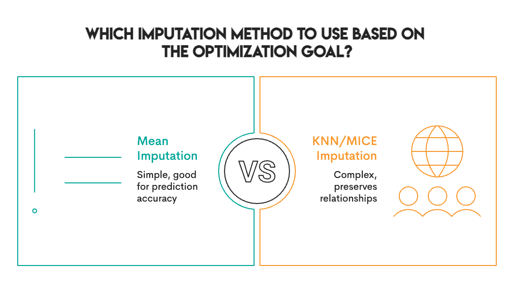
Photo by author
If you just need predictions, start simple. Test if KNN or RATS actually helps your data. Don’t assume they will.
If you need the correlation structure for downstream analysis, mean will quietly destroy it while giving you reasonably accurate numbers. It’s a trap.
And whatever you do, measure your properties before using KNN. Trust us on this.
Nate Rosedy A data scientist and product strategist. He is also an adjunct professor teaching analytics, and the founder of StrataScratch, a platform that helps data scientists prepare for their interviews with real interview questions from top companies. Netcareer writes on the latest trends in the market, gives interview tips, shares data science projects, and covers everything SQL.