


Photo by author
# Introduction
Most data scientists learn. Pandey By reading the lesson and copying the worked examples.
This is fine to start with, but it often results in bad habits among beginners. Use of iterrows() Loops, intermediate variable assignments, and repetition merge() There are some examples of calls code that is technically correct but is excessively slow and much harder to read than it should be.
The patterns below are not edge cases. They cover the most common day-to-day operations in data science, such as filtering, transforming, joining, grouping, and computing conditional columns.
In each of these, there is a shared perspective and a refined perspective, and the distinction is usually one of awareness rather than complexity.
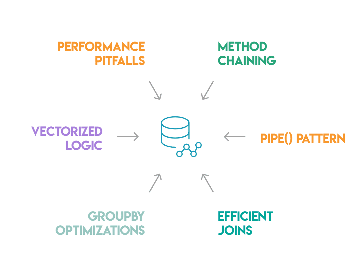
The six most influential are: method chaining, pipe() Patterns, efficient joins and merges, group by optimizations, vectorized conditional logic, and performance tradeoffs.
# The chain method
Intermediate variables can make code feel more organized, but often just add noise. The chain method Lets you write a series of transformations as a single expression, which reads naturally and avoids naming objects that don’t need unique identifiers.
instead of:
df1 = df(df('status') == 'active')
df2 = df1.dropna(subset=('revenue'))
df3 = df2.assign(revenue_k=df2('revenue') / 1000)
result = df3.sort_values('revenue_k', ascending=False)
You write this:
result = (
    df
    .query("status == 'active'")
    .dropna(subset=('revenue'))
    .assign(revenue_k=lambda x: x('revenue') / 1000)
    .sort_values('revenue_k', ascending=False)
)
Inside the lambda assign() Here is important.
When chaining, the current state of DataFrame Cannot be accessed by name; You must use a lambda to refer to it. The most common cause of broken chains is neglect, which usually results in a NameError or a stale reference to a variable that was previously defined in the script.
Another mistake to be aware of is usage. inplace=True within a chain. Methods with inplace=True return Nonewhich immediately breaks the chain. Place operations should be avoided when writing chained code, as they provide no memory benefit and make the code difficult to follow.
# pipe () pattern
When one of your transformations is complex enough to deserve its own separate function, using pipe() Allows you to keep it within the chain.
pipe() passes DataFrame As the first argument of any subscript:
def normalize_columns(df, cols):
    df(cols) = (df(cols) - df(cols).mean()) / df(cols).std()
    return df

result = (
    df
    .query("status == 'active'")
    .pipe(normalize_columns, cols=('revenue', 'sessions'))
    .sort_values('revenue', ascending=False)
)
It keeps the complex transformation logic inside a named, testable function while preserving chaining. Each piped function can be tested individually, something that becomes difficult when the logic is hidden within a wider chain.
The practical value of pipe() The appearance is spread out. Dividing the processing pipeline into labeled functions and linking them together pipe() Allows code to self-document. Anyone reading the sequence can understand each step by function name without needing to parse the process.
It also makes it easy to change or skip steps during debugging: If you comment pipe() Make the call, the rest of the chain will still run smoothly.
# Efficient joins and integrations
is one of the most commonly misused functions in Pandas. merge(). Two mistakes we often see are many-to-many joins and silent row inflation.
If both data frames have duplicate values in the join key, merge() Performs a Cartesian product of these rows. For example, if the join key is not unique on at least one side, then joining the 500-row “Customers” table to the “Events” table could result in millions of rows.
It makes no mistake. It produces only one DataFrame Which seems correct but is larger than expected until you examine its shape.
ok validate Parameter:
df.merge(other, on='user_id', validate="many_to_one")It raises a MergeError If multiple-to-one assumptions are violated. Use “one_to_one”, “one_to_many”, or “many_to_one” depending on what you expect from the join.
gave indicator=True The parameter is equally useful for debugging:
result = df.merge(other, on='user_id', how='left', indicator=True)
result('_merge').value_counts()
This parameter adds a. _merge Column showing whether each row comes from “left_only”, “right_only”, or “both”. This is the fastest way to catch rows that fail to join when you expect them to match.
In cases where both data frames share an index, join() is faster than merge() Because it works directly on the index instead of searching through a specific column.
# Group By Optimizations
When using a GroupByis a less used method. transform(). The difference between agg() And transform() It comes down to the shape you want back.
gave agg() method Returns one row per group. on the other hand, transform() Returns the same format as the original DataFrameeach row is filled with the total value of its group. This makes it ideal for adding group-level data as new columns without the need for a subsequent merge. It’s also faster from a manual aggregation and integration perspective because Pandas doesn’t need to align two data frames after the fact:
df('avg_revenue_by_segment') = df.groupby('segment')('revenue').transform('mean')It directly adds the average income of each segment in each row. Same result with agg() Using two steps instead of one, would require computing the mean and then recombining on the segment key.
For a key group by column, use ALWAYS. observed=True:
df.groupby('segment', observed=True)('revenue').sum()Without this argument, pandas computes results for each category specified in the column’s dtype, including combinations that do not appear in the original data. On large data frames with many categories, this results in empty groups and unnecessary calculations.
# Vectorized conditional logic
to use apply() with a Lambda function is the least efficient way to calculate the conditional values for each row. This avoids the C-level operations that pandas accelerates by running a Python function on each row independently.
For binary situations, NumPyOf np.where() A direct alternative is:
df('label') = np.where(df('revenue') > 1000, 'high', 'low')For several conditions, np.select() Handles them cleanly:
conditions = (
    df('revenue') > 10000,
    df('revenue') > 1000,
    df('revenue') > 100,
)
choices = ('enterprise', 'mid-market', 'small')
df('segment') = np.select(conditions, choices, default="micro")
gave np.select() The function maps the if/elif/else structure directly to vectorized trajectories by evaluating the conditions in sequence and assigning the first matching option. It is typically 50 to 100 times faster than the equivalent. apply() On one DataFrame With a million rows.
For numeric binning, the conditional assignment is completely reversed. pd.cut() (bins of equal width) and pd.qcut() (quantile-based bins), which automatically return a clear column without the need for NumPy. Pandas takes care of everything, including labeling and handling edge values, when you pass it the number of bins or bin edges.
# Performance losses
Some common patterns slow down Pandas code more than anything else.
For example, iterows() But it repeats DataFrame rows as (index, Series) pairs. This is an intuitive but slow method. for DataFrame With 100,000 rows, this function call can be 100 times slower than the vectorized equivalent.
The lack of performance comes from a complete build. Series object for each row and execute the Python code on it one at a time. Whenever you find yourself writing. for _, row in df.iterrows()stop and consider whether np.where(), np.select()or group by operation can replace it. Most of the time, one of them can do it.
to use apply(axis=1) is faster than iterrows() But shares the same problem: Python-level execution for each row. For every operation that can be represented by NumPy or pandas built-in functions, the built-in method is always faster.
Object dtype columns are also a convenient source of laziness. When Pandas stores strings as objects of dtype, operations on those columns are run in Python instead of C. For columns with low cardinality, such as status codes, region names, or categories, converting them to a categorical type can significantly speed up grouping and value_counts().
df('status') = df('status').astype('category')Finally, avoid chained assignments. to use df(df('revenue') > 0)('label') = 'positive' Can change initial DataFramedepending on whether Panda has created a copy behind the scenes. The behavior is undefined. use .loc Instead with a boolean mask:
df.loc(df('revenue') > 0, 'label') = 'positive'It is unambiguous and picks up numbers. SettingWithCopyWarning.
# The result
These patterns distinguish code that works from code that works well: efficient enough to run on real data, readable enough to maintain, and structured in a way that’s easy to test.
Method chain and pipe() Address readability, while join and group-by patterns address accuracy and efficiency. Vectorized logic and pitfall section address speed.
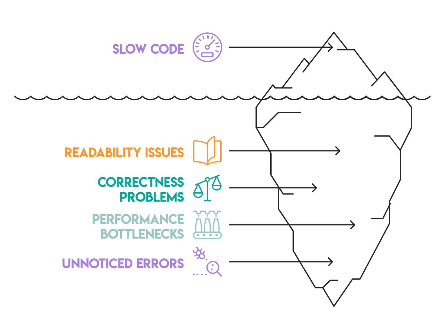
Most of the Panda code we review has at least two or three of these issues. They accumulate silently — a lazy loop here, an unverified merge there, or an object dtype column that no one noticed. None of them cause obvious failure, which is why they persist. Fixing them one at a time is a good place to start.
Net Rosiedi A data scientist and product strategist. He is also an adjunct professor teaching analytics, and the founder of StrataScratch, a platform that helps data scientists prepare for their interviews with real interview questions from top companies. Nate writes on the latest trends in the career market, gives interview advice, shares data science projects, and covers all things SQL.